神经网络

非线性假设 Non-linear Hypotheses

• 线性回归和逻辑回归的缺点：当特征数量很多时，计算负荷会非常大
• 神经网络可以很好地处理此类问题

模型表示

= activation of unit in layer
= matrix of weights controlling function mapping from layer to layer

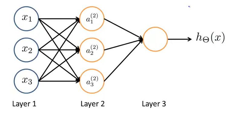
3 个激活单元表达式：

输出表达式：

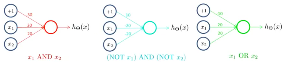
直观理解

代价函数

• 逻辑回归：
  
• 神经网络：
  $$h_{\Theta}(x) \in \mathbb{R}^{K} \quad\left(h_{\Theta}(x)\right){i}=i^{\text {th }}\text{output}\begin{aligned} J(\Theta)= & -\frac{1}{m}\left[\sum{i=1}^{m} \sum_{k=1}^{K} y_{k}^{(i)} \log \left(h_{\Theta}\left(x^{(i)}\right)\right){k}+\left(1-y{k}^{(i)}\right) \log \left(1-\left(h_{\Theta}\left(x^{(i)}\right)\right){k}\right)\right] \ & +\frac{\lambda}{2 m} \sum{l=1}^{L-1} \sum_{i=1}^{s_{l}} \sum_{j=1}^{s_{l+1}}\left(\Theta_{j i}^{(l)}\right)^{2}\end{aligned}$$

前向传播与反向传播公式推导

《 Neural Network and Deep Learning 》 - Chapter 2

Q：在拥有训练集输入 和输出 的情况下，我们应该如何调整网络参数 ，使模型的输出值与训练集的 尽可能接近？

前向传播过程

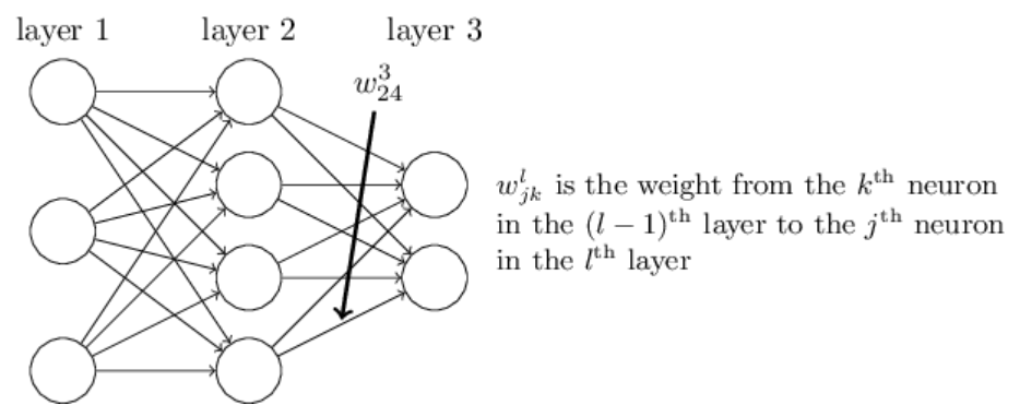
将上式重写为矩阵形式：

为方便表示，记：

反向传播过程

反向传播算法的直观理解： 和 描述了代价函数随权重 和偏置 变化而变化的程度。根据 和 以不断调整 和 ，从而使代价函数的值不断降低。

反向传播的两个假设

假设1：cost can be written as a function of the outputs from the neural network, for example：

假设2：总体代价函数可以表示为单个代价函数之和的平均

反向传播的四个方程

在计算 和 之前，首先引入中间量 （error in the neuron in the layer）。

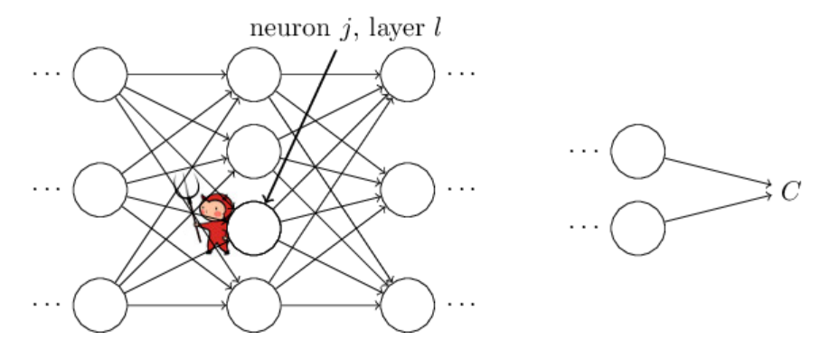
假设在神经网络模型中有一个捣乱的小恶魔，它让某个神经元的输入变化了 ，使得这个神经元的输出从原先的 变为了 。然后这个误差不断向前逐层传播，并导致最终的代价函数变化了 。

作为一个好恶魔，小恶魔很想弥补它的过错。当 是一个很大的值时，小恶魔可以选择一个和 相反的 ， 从而使代价函数降低。而当 已经接近于 0 时，不管小恶魔如何调整 ，最终代价函数的值都不会有太大的变化，因此这时小恶魔可以认为它已经找到“最优解”了。

So there’s a heuristic sense in which is a measure of the error in the neuron. Backpropagation will give us a way of computing for every layer, and then relating those errors to the quantities of real interest, and .

1. 输出层误差方程：
   
2. 误差传递方程：
   
3. 偏置的改变率：
   
4. 权重的改变率：